The idea of this notebook is to explore a step-by-step approach to create a single layer neural network without the help of any third party library. In practice, this neural network should be useful enough to generate a simple non-linear regression model, though it’s final goal is to help us understand the inner workings of one.
1. Working Data
First we will create a secret function that will generate a test score based on students hours of sleep and study. Note that in real life scenarios not only these secret functions will be unknown but in practice they usually dont exist, meaning, underlying relations between variables such as a Sleep and Study is far more complex and cannot be defined by a simple continuous function.
Additionally, as we will later observe, we expect that our neural network should provide us good approximations or predictors of the score but the actual secret function will remain unknown. In other works, we will only have a different, complex continuous function in which its output should be enough to approximate the original one.
# Our secret function
secretFunction <- function(x) {
  y <- (x[,1]^2 + x[,2]^2)
  return(t(t(y)))
}
Let’s assume a sample of 9 students, where each one had 3 days (72 hours) prior to the test and they either slept or studied.
# Our train (X) and test (xTest) data
Study <- round(runif(9,1,24))
Sleep <- 72 - Study
X <- data.frame(Study=Study,Sleep=Sleep)
xTest = rbind(c(3,7),c(2,8))

# We generate our Y train (y)
y <- secretFunction(X)
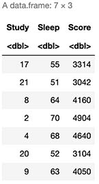
# This is our Study, Sleep and Score table
cbind(X,Score=y)
2. Generating the model
2.1 Functions
First, we need some functions to be defined:
- Rand: Generate random numbers
- Sigmoid: Our non-linear activation function to be executed by our Sigmoid neuron.
- Forward: Our forward propagation function.
- Sigmoid Prime: Gradient of our Sigmoid function for Backward Propagation.
- Cost: Cost calculation funtion (sum of squared errors)
# Random Function
rand <- function(x) {
  return(runif(1, 5, 100)/100)
}

# Sigmoid Function
sigmoid <- function(x) {
  return(1/(1+exp(1)^-x))
}

# Forward Propagation Function
Forward <- function(X,w1,w2) {
  X <- cbind(X[,1],X[,2])
  z2 <- X %*% w1
  a2 <- sigmoid(z2)
  z3 <- a2 %*% w2
  yHat <- sigmoid(z3)
  return(yHat)
}

# Sigmoid Gradient Function
sigmoidPrime <- function(x) {
  return((exp(1)^-x)/(1+(exp(1)^-x))^2)
}

# Cost Function
cost <- function(y,yHat) {
  sum(((yHat-y)^2)/2)
}
2.2 Parameter Initialization
Next, we need to define our parameters. We have two sets of parameters:
- Hyperparameters: Parameters that the network cannot learn and are pre-defined.
- Number of hidden layers: In this case we have 1, since it’s a simple single layered neural network.
- Number of Neurons of hidden layers: We will use 6.
- Learning Rate: We will use 2.
- Learning Parameters: Parameters that our network will learn.
- Weights: We will use 2 weights since by design we will need at leas N+1 weights where N is equivalent to the number of Hidden Layers.
# Hyperparameters
inputLayerSize = ncol(X)
outputLayerSize = 1 # Dimension of outputs (1 since it's only score)
hiddenLayerSize = 6 # Number of neurons
LearningRate <- 2

# Weights
w1 <- matrix(runif(inputLayerSize*hiddenLayerSize), nrow = inputLayerSize, ncol = hiddenLayerSize )
w2 <- matrix(runif(hiddenLayerSize*outputLayerSize), nrow = hiddenLayerSize, ncol = outputLayerSize )
2.3 Data Normalization
# We normalize train data
X = X/max(X)
y = y/max(y)

# We normnalize test data
xTest <- xTest/max(X)
yTest <- secretFunction(xTest)/max(y)
3. Propagation
3.1 Forward Propagation
# We propagate
yHat <- Forward(X,w1,w2)
3.1.1 Cost Calculation
# We calculate cost
J <- sum(((yHat-y)^2)/2)
J

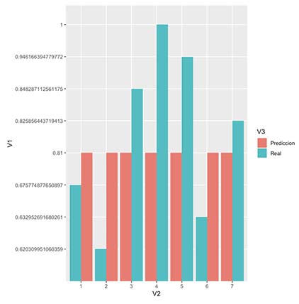
3.1.2 We evaluate the results
library(ggplot2)
resultPlot <- as.data.frame(rbind(cbind(y,1:nrow(y),"Real"),cbind(round(yHat,2),1:nrow(yHat),"Prediccion")))
ggplot(resultPlot, aes(x=V2, y=V1, fill=V3)) + geom_bar(stat="identity", position="dodge")
3.2 Back propagation
# We derivate W2 in respect to the cost
dJdW2 <- function(X,w1,w2) {
  X <- cbind(X[,1],X[,2])
  z2 <- X %*% w1
  a2 <- sigmoid(z2)
  z3 <- a2 %*% w2
  yHat <- sigmoid(z3)
  delta3 <- -(y-yHat)*sigmoidPrime(z3)
  cost <- t(a2) %*% delta3
  return(cost)
}

# We adjust W2
w2 <- w2 - (LearningRate * dJdW2(X,w1,w2))

# We derivate W1 in respect to the cost
dJdW1 <- function(X,w1,w2) {
  X <- cbind(X[,1],X[,2])
  z2 <- X %*% w1
  a2 <- sigmoid(z2)
  z3 <- a2 %*% w2
  yHat <- sigmoid(z3)
  delta3 <- -(y-yHat)*sigmoidPrime(z3)
  delta2 <- (delta3 %*% t(w2)) * sigmoidPrime(z2)
  cost <- t(X) %*% delta2
  return(cost)
}
w1 <- w1 - (LearningRate * dJdW1(X,w1,w2))
3.3 We forward propagate again
# We propagate Again!
yHat <- Forward(X,w1,w2)
3.3.1 New Cost Calculation
# We calculate cost
J <- sum(((yHat-y)^2)/2)
J

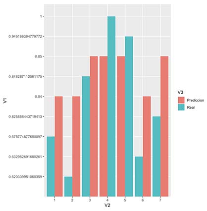
Note: We should observe a small improvement in cost due to the new parameters.
3.3.2 We evaluate again
library(ggplot2)
resultPlot <- as.data.frame(rbind(cbind(y,1:nrow(y),"Real"),cbind(round(yHat,2),1:nrow(yHat),"Prediccion")))
ggplot(resultPlot, aes(x=V2, y=V1, fill=V3)) + geom_bar(stat="identity", position="dodge")
4. Backpropagate, Forwardpropagate and repeat
We will now repeat the previous process until we cannot minimize our cost any more. When this happens, it means we have found a local minima. We will stop when we observe that error calculated at step n+1 is equal or superior than the one found in step n, meaning we cannot improve any more with out jumping around the local minima.
costTrain <- data.frame(Training=NA,Cost=NA)
costTest <- data.frame(Training=NA,Cost=NA)
InitialError <- sum((y-yHat)^2)
FinalError <- 0
i <- 1

while(round(FinalError,5) <= round(InitialError,5)) {
  w1 <- w1 - (LearningRate * dJdW1(X,w1,w2))
  w2 <- w2 - (LearningRate * dJdW2(X,w1,w2))
  yHat = Forward(X,w1,w2)
  costo <- cost(y,yHat)

  costTrain[i,]$Training <- i
  costTrain[i,]$Cost <- costo

  FinalError <- sum((y-yHat)^2)

  i <- i + 1
  if(i %% 1000==0) {
    # Print on the screen some message
    cat(paste0("Iteration ", i,": ",FinalError,"\n"))
  }
  if(i == 30000) {
      break()
  }
}

4.1 We evaluate again
library(ggplot2)
resultPlot <- as.data.frame(rbind(cbind(y,1:nrow(y),"Real"),cbind(round(yHat,2),1:nrow(yHat),"Prediccion")))
ggplot(resultPlot, aes(x=V2, y=V1, fill=V3)) + geom_bar(stat="identity", position="dodge")
Improvement <- (InitialError-FinalError)/InitialError
cat(paste("Initial Error: ",InitialError,"
Final Error: ",FinalError,"
Improvement: ",round(Improvement,2)*100,"%
Took ",i," Iterations",sep=""))
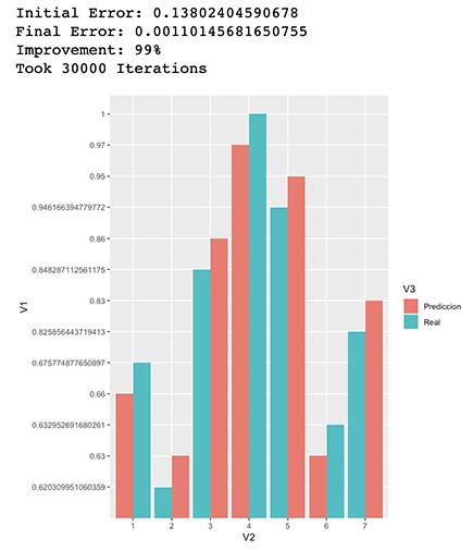
As seen in the results above it seems our model was able to predict very similar scores to our “Secret Function”, even though the actual model is a mix of a more complex combination of vector products and non-linear functions. This means our new model approximates quite well our actual “Secret Function Model”.
5. How our training improved our model?
costTrain$Data <- "Train"
ggplot(costTrain, aes(x=Training, y=Cost)) + geom_line()
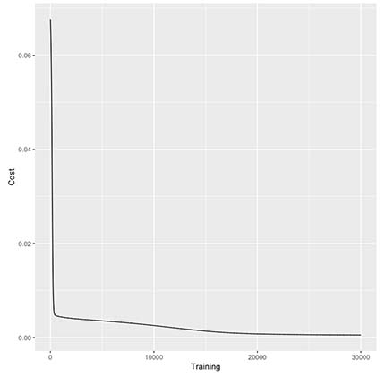
As seen above it seems there’s only small costs improvements after every 1k iterations.
6. Evaluation on known (in sample) Data
Train <- X
# Note: this output represents a normalized representation of Study and Sleep
cbind(Train,RealScore=secretFunction(Train),PredictedScore=Forward(Train,w1,w2))
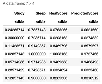
Lets translate this to our original scale
Since all our inputs are normalized our outputs will also be decimals within a 0 and 1. Due to this, we need to “denormalize” our results.
X <- data.frame(Study=Study,Sleep=Sleep)
y <- secretFunction(X)
cbind(X,Score=secretFunction(X),Prediction=round(Forward(Train,w1,w2)*max(y)))
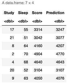
As expected, it seems our model provide us very good approximations to actual test scores.
7. Evaluation on unknown (out of sample) data
7.1 Original (Secret) Function
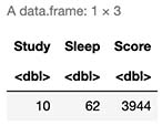
Let’s evaluate which test score we should expect from a student who studied 10 hours and slept 62. This can be done by executing our “Secret Function” as follows:
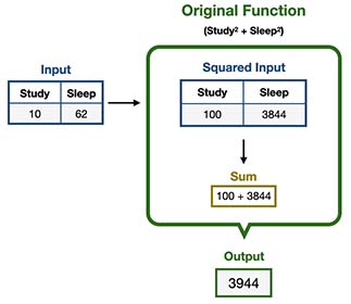
It’s important to remember that normally we do not have access to this nor any underlying function, since most likely they not even exists.
Alternatively in R:
xTrain <- data.frame(Study=16,Sleep=56)
yTrain <- secretFunction(xTrain)
cbind(xTrain,Score=yTrain)
7.2 New Learned Function
We will try to predict the score for this student using our new Learned Function. You’ll notice that this function is far more complex than our original -allegedly unknown- one, though its output approximates quite well our original results.
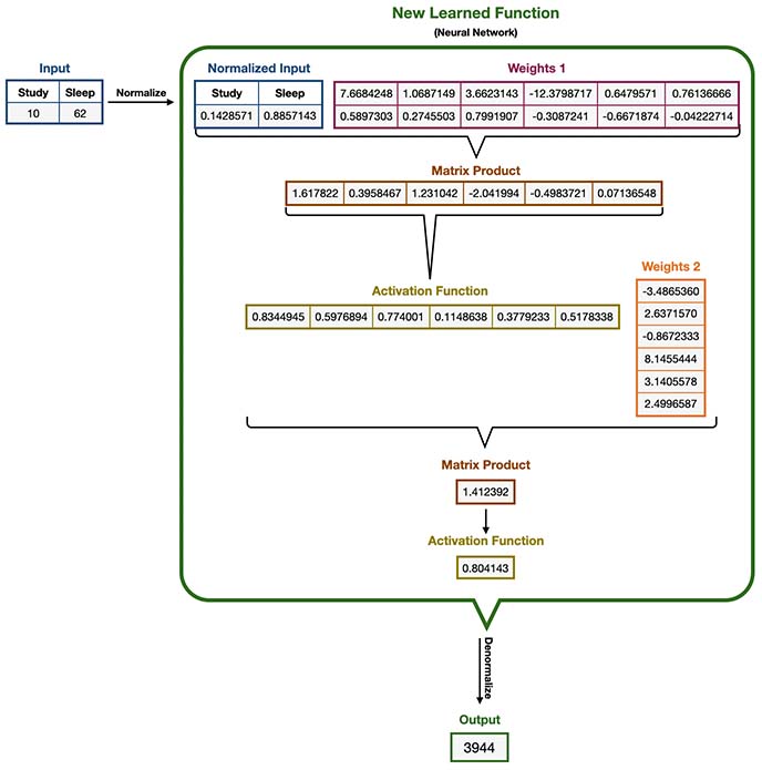
As you might have noticed, this function is sometimes called a “black box” function, since it’s quite difficult to interpret; we just cannot easily observe any underlying relationship. In contrast, in our original function, we can observe that students score was directly proportional to both Sleep and Study and in fact was the sum of its squares.
Alternatively in R:
as.integer(round(Forward(xTrain/max(X),w1,w2)*max(y)))
![]()
Seems our predicted score it’s the same as the original one (3944), which is great!
Simulation: How our model predicts new data
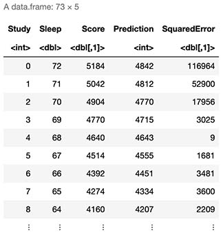
Lets simulate 72 students, starting from a student who studied 0 hours and slept 72, up to the opposite scenario.
Test <- data.frame(Study=seq(0,72))
Test$Sleep <- 72-Test$Study
Test$Score <- secretFunction(Test)
Test$Prediction <- as.integer(round(Forward(Test/max(X),w1,w2)*max(y)))
Test$SquaredError <- (Test$Score - Test$Prediction)^2
Test
8. Final Thoughts
Let’s see how well our model predicts outside our training space.
ggplot(Test, aes(x=Study, y=sqrt(SquaredError))) +
    geom_line() +
    geom_vline(xintercept=min(X$Study), linetype="dashed", color = "red") +
    geom_vline(xintercept=max(X$Study), linetype="dashed", color = "red")
cat(paste("Training Space Known by model:\n   Min Study Hours:",min(X$Study)),"\n   Max Study Hours:",max(X$Study))
RMSEWithin <- round(sqrt(mean(Test$SquaredError[which(Test$Study >= min(X$Study) & Test$Study <=max(X$Study))])))
RMSEBelow <- round(sqrt(mean(Test$SquaredError[which(Test$Study < min(X$Study))])))
RMSEAbove <- round(sqrt(mean(Test$SquaredError[which(Test$Study > max(X$Study))])))
cat(paste("\n\nAverage Root Mean Squared Error:\n   Below Known Range:",RMSEBelow, "\n   Within Known Range:",RMSEWithin,"\n   Above Known Range:",RMSEAbove))
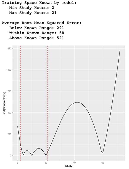
As observed by the errors from the table and the plot above, it seems that our new function had somewhat better prediction capabilities within the training space which is represented by our vertical lines. As expected, our new model is not able to predict out-of-sample data that falls outside of our training space since our calculated costs start to increase and behave erratically.
In other words, our model is able to interpolate quite well the approximation of Students score by providing their time of Study and Sleep, in contrast, is not able to extrapolate very well outliers or data outside its training space.
